The discrete Fourier transform, or DFT, is the primary tool of digital signal processing. The foundation of the product is the fast Fourier transform (FFT), a method for computing the DFT with reduced execution time. Many of the toolbox functions (including Z -domain frequency response, spectrum and cepstrum analysis, and some filter design and implementation functions) incorporate the FFT.
The MATLAB® environment provides the functions fft and ifft to compute the discrete Fourier transform and its inverse, respectively. For the input sequence x and its transformed version X (the discrete-time Fourier transform at equally spaced frequencies around the unit circle), the two functions implement the relationships
X ( k + 1 ) = ∑ n = 0 N - 1 x ( n + 1 ) W N k n
x ( n + 1 ) = 1 N ∑ k = 0 N - 1 X ( k + 1 ) W N - k n .
In these equations, the series subscripts begin with 1 instead of 0 because of the MATLAB vector indexing scheme, and
W N = e - j 2 π / N .
Note The MATLAB convention is to use a negative j for the fft function. This is an engineering convention; physics and pure mathematics typically use a positive j .
fft , with a single input argument, x , computes the DFT of the input vector or matrix. If x is a vector, fft computes the DFT of the vector; if x is a rectangular array, fft computes the DFT of each array column.
For example, create a time vector and signal:
t = 0:1/100:10-1/100; % Time vector x = sin(2*pi*15*t) + sin(2*pi*40*t); % Signal
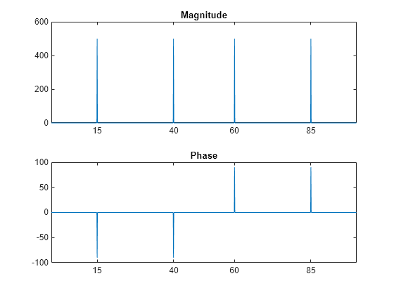
Compute the DFT of the signal and the magnitude and phase of the transformed sequence. Decrease round-off error when computing the phase by setting small-magnitude transform values to zero.
y = fft(x); % Compute DFT of x m = abs(y); % Magnitude y(m<1e-6) = 0; p = unwrap(angle(y)); % Phase
To plot the magnitude and phase in degrees, type the following commands:
f = (0:length(y)-1)*100/length(y); % Frequency vector subplot(2,1,1) plot(f,m) title('Magnitude') ax = gca; ax.XTick = [15 40 60 85]; subplot(2,1,2) plot(f,p*180/pi) title('Phase') ax = gca; ax.XTick = [15 40 60 85];

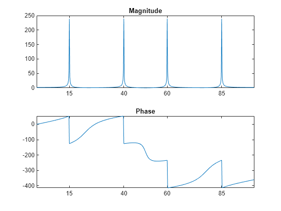
A second argument to fft specifies a number of points n for the transform, representing DFT length:
n = 512; y = fft(x,n); m = abs(y); p = unwrap(angle(y)); f = (0:length(y)-1)*100/length(y); subplot(2,1,1) plot(f,m) title('Magnitude') ax = gca; ax.XTick = [15 40 60 85]; subplot(2,1,2) plot(f,p*180/pi) title('Phase') ax = gca; ax.XTick = [15 40 60 85];

In this case, fft pads the input sequence with zeros if it is shorter than n , or truncates the sequence if it is longer than n . If n is not specified, it defaults to the length of the input sequence. Execution time for fft depends on the length, n , of the DFT it performs; see the fft reference page for details about the algorithm.
Note The resulting FFT amplitude is A*n/2 , where A is the original amplitude and n is the number of FFT points. This is true only if the number of FFT points is greater than or equal to the number of data samples. If the number of FFT points is less, the FFT amplitude is lower than the original amplitude by the above amount.
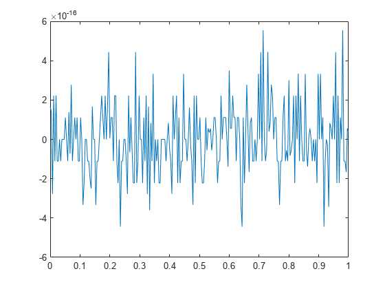
The inverse discrete Fourier transform function ifft also accepts an input sequence and, optionally, the number of desired points for the transform. Try the example below; the original sequence x and the reconstructed sequence are identical (within rounding error).
t = 0:1/255:1; x = sin(2*pi*120*t); y = real(ifft(fft(x))); figure plot(t,x-y)

This toolbox also includes functions for the two-dimensional FFT and its inverse, fft2 and ifft2 . These functions are useful for two-dimensional signal or image processing. The goertzel function, which is another algorithm to compute the DFT, also is included in the toolbox. This function is efficient for computing the DFT of a portion of a long signal.
It is sometimes convenient to rearrange the output of the fft or fft2 function so the zero frequency component is at the center of the sequence. The function fftshift moves the zero frequency component to the center of a vector or matrix.